Showing posts with label Computing. Show all posts

Wednesday, February 26, 2014

On the computer languages market

There is an interesting series of articles on Dr. Dobb's essentially about what we can call the computer languages market, where they analyze trends and caracteristics, especially in the Editor in chief's article.

They analyze the trends in language usage, which ordinally had not change since the year before (C, Java, Objective-C, C++, C#, PHP, Visual Basic, Python and Javascript), but that show a number of developments. For instance, Perl is leaving room in favor of Python. Perl seems to be dying and with signs of becoming history. They also mentioned a strong resurgence of Javascript but I would like to add that a large number of developments in the web scripting world have been carried out, starting with CoffeeScript, a tiny language that translates 1-to-1 to JavaScript. See their web page for some use of the language. ClojureScript is another compiler, this time to translate Clojure into JavaScript.

I found the following paragraph of particular interest:
By all measures, C++ use declined last year, demonstrating that C++11 was not enough to reanimate the language's fortunes, despite the significant benefits it provides. I have previously opined that Microsoft's contention of a return to native languages being led by C++ was unsupported by evidence. It is now clearly contradicted by the evidence.
I feel encouraged by this statement. I believed C++ is an awful language, and always has been. Back in the late 90's when I started programming and my teenage budget in a remote outpost included a non-disposable 486 DX2 with DOS, we had no choice but to get mainstream technical stuff, and that included C++ as the only advanced systems language. My experience, and I believe everybody's experience, is that programmer's time is more important than running time, and even hardcore C++ programmers recognize they put themselves in pain when facing non-standard tasks with the language. Some would argue that pain is what you pay for system performance, but that is not true (see the paragraph below). C++ will never grow on Big Data (data processing), mobile development or cloud computing, and I would expect that performance computing to also cut C++ usage in favor of more modern, maintainable system languages, such as the D language (or the one I describe below).

An interesting development they had not talked about in the area of systems programming, more than the D language, is Nimrod. It has cool features such as pointers that are traced by a lightweight garbage collector and others that directly translate to C++ pointers. Templates that can be called as operators are included, supporting metaprogramming, it supports inmutable objects, a number of syntactic sugars (such as being able to call len(x), x.len or x.len if there is only one argument, command and function-like calls like echo("hello") and echo "hello"...), first class functions and a very good mixture between Python indentation-defined blocks and Scala function definitions, as opposed to D's C-like syntax. Nimrod compiles to C, C++, Objective C and JavaScript. Definitely a good candidate to learn and to watch.

On the functional but high-performant side of the market we have Erlang, Haskell, Scala and Clojure. The first three are older, especially the first two ones. In my opinion, Clojure is simplest, especially when compared to Scala. This is patent when examining a source coude listing in both languages. Clojure lifts the programmer's productivity to new highs (I was able to code the Denarius' matching engine core in half a day). Definitely the way to go in the future.

Saturday, February 1, 2014

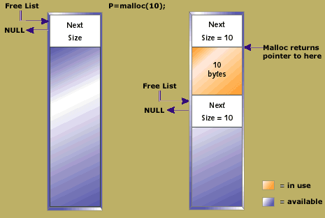
What lies underneath malloc

malloc is C's dynamic memory allocation function: memory is assigned to the process heap and then the malloc dynamic assignation does its magic, to make boundaries between dynamically assigned variables. Here's how it works (bear in mind that a malloc implementation is largely compiler-dependent):

At the beginning of the process' heap free space, a special region is allocated to point to the next available byte address in the free region and a previous pointer to the pointers corresponding to the previously allocated block. In case there is no block allocated next, the pointer is null. Otherwise, the pointer will point as many bytes ahead in the process memory as the corresponding allocated block's size.

The function free updates the following block's previous pointer after the recently liberated block, which causes mismatch with the preceding block's next pointer pointing to the deleted block. This creates an accounted free block. To speed up, free can have its own list of free block and sizes elsewhere on the heap.

Tuesday, December 17, 2013

Damn, Clojure is fast!

Well I feel positive today, I struggled for the past two days to make my logistic regression in Clojure faster. I even made up to four different implementations of the logistic regression, with none of them giving satisfactory results. It all was even more disappointing when comparing to my MyML logistic regression implementation.

Well, I found out what the problem was: Actually I was making two fatal errors.
  • My input data in Clojure were lists instead of vectors
  • My input data in Python was 256 datapoints, instead of 1000 as in the Clojure version.
Both points stemmed from me being not so careful. In the first case, I knew already that one should use vectors instead of list when going after performance, but I was assuming that my data was in vector form. Staring at the variable X, I wondered if it was vector or list and voila, performance just got x5 better. Then I went to the Python interpreter, checked whether the number of iterations in the gradient descent object was the same as in Clojure, and then checked the data... well, my data was smaller (from a previous test with logistic regression). I re-generated my data and Python just lagged behind. In particular, I give you the figures (notice that I did not bother to put the wrong results I was getting because of my mistakes):

Python: 0.56 sec
Clojure: 0.19 sec (iterative implementation through loop-recur) 0.04 sec (concurrent implementation through agents).

Bear in mind that I am conduncting the tests on my girlfriend's borrowed machine and that I installed Cristoph Gohlke's Numpy distribution, which shippes with Intel's MKL statically-linked libraries, so it should be pretty fast in terms of algebraic computations. Perhaps the lack of performance comes from Python's interpreter itself (read-interpret-execute...). This is even more supporting of Clojure, since we are focusing on the infrastructure of both systems.

I will be putting everything in order, making my logistic regression more idiomatic and building some tests.

Monday, October 21, 2013

Clojure structures, deconstruction and higher-order functions to make our lives better

Clojure provides an easy and more productive way of writing programs and it is available to us if we want to stay away from the common imperative, sequential, start-to-end way of thinking.

During my time as a developer, both (and especially) in the academia and in production software, I've come across the problem of getting the index of those elements in an array that meet a constrain. This is easy (although after some training, as usual) in Clojure
(defn index-filter [pred coll]
  (for [[i elem]
    (map-indexed (fn [a b] [a b]) coll) :when (pred elem)]
   i))
The way this works is: the for macro associates each i and elem  to the pairs in the sequence given by (fn [a b] [a b]) coll). This is filtered by executing the predicate on each element. The predicate, in turn, filters out the elements in which we are not interested. The for body then returns each of the index that passed the condition.

We can separate the functionality into two functions, the first to write the indexing of the original elements as an independent function:
(def make-index (partial map-indexed (fn [a b] [a b]) ))
We use (partial) to make a function that still needs an input argument and associate it into the make-index symbol. Placing it into the general code:
(defn index-filter [pred coll]
  (for [[i elem] (make-index coll) :when (pred elem)]
   i))
The way you call this function is with a predicate and a collection. For example, Now we have a very elegant solution that is valid for many data types.

Wednesday, September 11, 2013

Load Kaggle datasets directly into Amazon EC2

Despite not having access to a suitable environment at home, I decided to enter a new Kaggle competition. The StumbleUpon Evergreen Classification Challenge seems to be easy to tackle since it is a classic binary classification problem with text features and numerical features.

I decided to do it on the cloud. For that purpose, one needs to load the data distributed by Kaggle into the Amazon EC2 instance. Kaggle will prevent any connection from there, since they require you to log in to access the data. No problem, it is the cookies which do the work, and we are going to use them from the EC2 instance, as they commented here

The first thing we need is a plugin to save the cookies into a text file. Use this for Firefox, and this for Chrome.

Then, we upload the file to the EC2 instance with some means. In my case I use Bittorrent Sync (a post will be coming later on). We tell wget to use the cookies with the option --load-cookies as this:

wget -x --load-cookies ~/BTSync/cookies.txt http://www.kaggle.com/c/stumbleupon/download/raw_content.zip

We get an output such as this, and we have successfully loaded the data:

ubuntu@ip-172-31-21-138:~/kaggle/evergreen$ wget -x --load-cookies ~/BTSync/cookies.txt http://www.kaggle.com/c/stumbleupon/download/raw_content.zip
--2013-09-09 22:37:17--  http://www.kaggle.com/c/stumbleupon/download/raw_content.zip
Resolving www.kaggle.com (www.kaggle.com)... 168.62.224.124
Connecting to www.kaggle.com (www.kaggle.com)|168.62.224.124|:80... connected.
HTTP request sent, awaiting response... 302 Found
Location: https://kaggle2.blob.core.windows.net/competitions-data/kaggle/3526/raw_content.zip?sv=2012-02-12&se=2013-09-12T22%3A37%3A18Z&sr=b&sp=r&sig=qAJZIFUmRu%2B9XX%2FM%2B7qPorR%2FkWAC7%2B9W6MEWL5xM0fg%3D [following]
--2013-09-09 22:37:18--  https://kaggle2.blob.core.windows.net/competitions-data/kaggle/3526/raw_content.zip?sv=2012-02-12&se=2013-09-12T22%3A37%3A18Z&sr=b&sp=r&sig=qAJZIFUmRu%2B9XX%2FM%2B7qPorR%2FkWAC7%2B9W6MEWL5xM0fg%3D
Resolving kaggle2.blob.core.windows.net (kaggle2.blob.core.windows.net)... 65.52.106.46
Connecting to kaggle2.blob.core.windows.net (kaggle2.blob.core.windows.net)|65.52.106.46|:443... connected.
HTTP request sent, awaiting response... 200 OK
Length: 164757969 (157M) [application/zip]
Saving to: ‘www.kaggle.com/c/stumbleupon/download/raw_content.zip’

100%[======================================>] 164,757,969 2.29MB/s   in 95s

2013-09-09 22:38:53 (1.65 MB/s) - ‘www.kaggle.com/c/stumbleupon/download/raw_content.zip’ saved [164757969/164757969]

ubuntu@ip-172-31-21-138:~/kaggle/evergreen$

Monday, September 9, 2013

Stuff: Cook computers in the oven to resucitate them and cool Windows account hacking

I wanted to share a couple of experiences with computers that I have had in the period of one week.

A couple of weeks ago a number of friends and I went on vacations and we rented a house in the middle of nowhere. We brought a Wifi router and our laptops and played a very old computer game that everybody still loves, which is Age of Mythology.

At the end of our stay, one of my laptops (the old one) stopped working, and my friends told me the last thing it did was painting strange lines along with the graphics, i.e., a graphics card issue. I must say that this comes at an already tumultous time between me and technology, since my new laptop just died some time ago and it's in repair.

When we got home, I looked for information on the possible issue. And I came across this

The funny thing is: IT WORKS!

We removed the NVidia video card, put it in the oven as it says, 8 min at 200 celsius, put it back on and voila! Graphics back!

The next experience was: I was given my sister's old laptop. It is old but still decent and she only changed laptop because the disk crashed... I took it and recovered her files later on. Anyway, it must be the two-year long rest but the disk is living now. The only problem: we could not access the laptop because of her password.


Here's Youtube to the rescue again. This, however, semms to only work with Windows 7 and 8, not with Vista, the one on the laptop. Anyway, we got the disk out, put it on my external drive case, and accessed the files from there. This hack works like this:
  • The accesibility button on the Windows log in screen (bottom left) calls a program called utilman.exe, located under C:\Windows\System32
  • Accessing the drive, we rename it to utilman1.exe and make a new copy of cmd.exe to utilman.exe, therefore utilman.exe is now a command prompt.
  • When we put the disk on again and started Windows, pressing the accessibility button shows a privileged command prompt. From there, we issued the command net user myuser x, effectively resseting the password to a plain x.
This left us with a ready to use laptop (not critial tasks, just online gaming), just what we needed for the afternoon

Addendum: I believe it is interesting if I mark the post with the laptop that was reflowed with this technique: This is an Acer 5920g and the NVidia card was a 8600M GT. Apparently, these NVidia processors (prior to 2009) have a problem with the heat from using them and the cooling down when not in use: This makes internal circuits break, much like a stone exposed to the sun. Heating them to over 200 celsius make the connections sufficiently liquid so as to resolder again.

Friday, August 2, 2013

Installing Theano on Windows 64 bit (x86_64) with GPU capabilities

Since Theano team works under Linux, those of us that bought a laptop with a fancy Windows version pre-installed and decided that we wanted some compatibility with technology-reluctant friends and family (therefore assuming difficulties with everything else), we are doomed to hack our way into getting Theano up and running.

In this post I assume you are going with Cristoph Gohlke's packages (for reasons, read a previous post)

Make sure you also have MS Visual C++ and the NVidia CUDA Toolkit. If you don't have it, add the Visual C++ cl.exe compiler's directory to the path. Mine was under C:\Program Files (x86)\Microsoft Visual Studio 10\VC\bin.

First think you need, after installing Theano, is the nose package, since Gohlke's build needs it at initialization time. Download it and install it from Gohlke's site along with Theano.

Next, you need this .theanorc to be put under your home directory under C:\USER\<yourname>
[global]device = gpu
[nvcc]compiler_bindir=C:\Program Files (x86)\Microsoft Visual Studio 10.0\VC\bin# flags=-m32 # we have this hard coded for now
[blas]ldflags =# ldflags = -lopenblas # placeholder for openblas support
I am not very sure how to use OpenBLAS from here. I assume that if all CPU operations are done via Numpy and SciPy, then their default BLAS routines are used, and no direct call to a third BLAS implementation is made, but who knows! (Well, I looked into it a little bit and it seems Theano calls BLAS directly, I guess you may want to install OpenBLAS).

OK, we have the NVidia compiler and tools, the MS compiler that nvcc needs and the configuration. The last thing we need is to install a GNU C and C++ compiler that supports 64 bit Windows binary creation. There is a project called MinGW-w64 that does that. I recommend to download a private build from the user rubenvb that does not come along with the Python environment embedded as the more official build does. Put the bin directory (where GCC is located) of that installation in the Path (Control panel, etc). Theano needs this to compile the symbolic operations to object code and then to CUDA kernels if applicable, I presume.

If you run into errors of type "GCC: sorry, unimplemented: 64-bit mode not compiled in", then your MinGW is not x86_64 compliant. The NVidia compiler nvcc can also complain if it finds no cl.exe in the path.

By the way, all of this was to use deep learning techniques for Kaggle competitions, so the intended consequence was to install PyLearn2. This is not listed under Gohlke's libraries, but it is not low level and all is based on Theano and maybe other numerical packages such as Numpy. Being a pure Python package, you need to clone it from Github:
git clone git://github.com/lisa-lab/pylearn2.git
And then perform
cd pylearn2
python setup.py install
There is an easier procedure that will not require you to manually perform the git operations, and it is through pip
pip install git+git://github.com/lisa-lab/pylearn2.git
You have pip under your Python installation, within the Scripts directory, in the case it came with Python, or if you got Gohlke's installer.

This will also leave the module correctly accessible through Python.

Edit: Pylearn2's tutorial test is a little bit complicated to be a "hello world" test, so I looked for another quick example to see if my installation was finished. A very nice one popped up in this link, which I reproduce here. But first I have to tell that this made me realize that Gohlke's Theano is missing three files, something very, very strange since they are called from within Theano. In particular, the module missing is everything under theano.compat. In this case, just copy the contents from Theano's Github repository directory compat to a compat directory created on your local theano installation under Python 2.7 (mine C:\Python27\Lib\site-packages\theano).

After that, run the code in this link, which is a neural network solving the XOR problem. And we are done.

MinGW-w64: rubenvb build.
Python libraries and builds for Windows: Cristoph Gohlke.
Link to a "truer" hello world Pylearn2 program: here.

Monday, July 29, 2013

Mathematical analysis of MapReduce

Everybody is talking about MapReduce. They talk a lot about it even though they barely know what it is. I guess they talk about it because of all Google hype.

To put it simply, MapReduce is
$$\left. F (f_y)  \right|_{y=k}$$

where the function $f$ is the map, $ F $ is the reduce and $k$ is the key. In the special case the reduce just adds the values, the above becomes
$$\left. \int f_y (x) dx \right|_{y=k}$$
where $x$ are the values and $F$ is a linear functional (i.e., an element of the algebraic dual of the space where $f_y$, for all $y$ -the keys-, live.

The prominent example of computing the maximum temperatures from "Hadoop: The definitive guide" is the operation
$$\left. \| f_y \|_{\infty} \right|_{y=k}$$


It is "just" an abstraction of a basic operation found ubiquitously.

Tuesday, April 30, 2013

Hadoop "Incompatible namespaceIDs" error

This is an error that I faced a while ago and I made a blog entry to be publised some day, so here it goes.

When setting up an installation and if not everything goes well, we might face the situation of datanode/namenode desyncrhonization. You should immediately refer to the logs. There you can see the following message:
 ... ERROR org.apache.hadoop.dfs.DataNode: java.io.IOException: Incompatible namespaceIDs in /app/hadoop/tmp/dfs/data: namenode namespaceID = 308967713; datanode namespaceID = 113030094
        at org.apache.hadoop.dfs.DataStorage.doTransition(DataStorage.java:281)
        at org.apache.hadoop.dfs.DataStorage.recoverTransitionRead(DataStorage.java:121)
  1. Go to you namenode's directory (dfs.name.dir) and get the namespaceID value from current/VERSION.
  2. Go to your data node's storage directory (dfs.data.dir) and edit current/VERSION.
  3. Change the value to the datanode's value for the namenode's value.


I had not been able to repair the filesystem with any other way.

Saturday, December 22, 2012

Funny Boost

I located some examples I made when I first got acquainted with Boost and wanted to push the limits of the tutorials. Imagine the following two flavors of a program:
#include <boost/smart_ptr/shared_ptr.hpp>
using namespace std;
using namespace boost;
struct Thing {
public :
    Thing(int *i);
    void dumpP() {cout << pInt.get() << endl;}
private:
    shared_ptr<int> pInt;
};
Thing::Thing(int *i) : pInt(i) {
}
int _tmain(int argc, _TCHAR* argv[])
{
    int i;
    Thing t(&i);
    cout << &i << endl;
    t.dumpP();
   
    std::cin >> i;

    return 0;
}
 And
#include <boost/smart_ptr/shared_ptr.hpp>
using namespace std;
using namespace boost;
struct Thing {
public :
    Thing(int *i);
    void dumpP() {cout << pInt.get() << endl;}
private:
    shared_ptr<int> pInt;
};
Thing::Thing(int *i) : pInt(i) {
}
int _tmain(int argc, _TCHAR* argv[])
{
    int *j = new int(1);
    Thing t(j);
    cout << j << endl;
    t.dumpP();

    std::cin >> *j;

    return 0;
}
We see that their only difference is the fact that in the first version we use a local variable and in the second we allocate memory. Both are syntactically correct and both compile. However, one of them crashes before finishing execution.

If your guts tell you it is the one that uses dynamic memory, it is betraying you. The one that fails is the version that uses the local variable. What's the harm?

When they are deleted, Boost "intelligent" pointers free the object they reference if they are the last referencing pointer. This assumes the pointer is a dynamically-allocated variable. Since in the first version the variable is contained in the stack and has no valid dynamic memory block pointers, this crashes the program when it tries to free that part of the memory. This also explains why the last version works.

Tuesday, September 18, 2012

Python IDE: Spyder

I've been working with the Spyder IDE for Python. It is time I share my impressions.

First of all, it is a very strange feeling what you get when working with the IDE. In fact, it is the same feeling (but even more exaggerated) than you get with R Studio (in the case of programming for R). I feel like there is a force that prevents me from doing my work. In this regard, Spyder looks more like R Studio than to Matlab (a resemblance this last one that is the developers' motto).


I reckon that the IDE surpasses every other IDE that I've tried out so far, but there is still this unavoidable feeling. I think part of it comes from the fact that when you are executing part of the code just to see if it really does what it is intended for, it leaves the windows focus at the command line panel, and there is no keyboard combination to make it go back to the current file that is in edition. It is also possible that I am using Ubuntu and this software is more ready for KDE since it uses the Qt libraries.

On the other hand, you have the handy feature of integration with pdb, the Python debugger, showing variables of the current scope, an online help which shows documentation for any loaded name.

A fine IDE but that still needs maturing a little bit.

spyder-ide.blogspot.com

Saturday, August 4, 2012

Using whatsapp on your PC (II)

First of all, don't use cracks even if you find no virus. They use Whatsapp's verification of your phone number to send messages to I don't know who.

That being said, my fiancée Sali found what I had given all hope finding: a free and competitive Android emulator called Bluestacks App Player.

Even though it is little known, Bluestacks is the BEST Android emulator with a vengeance.

It runs Whatsapp seamlessly, totally recommended.

I know now what the rascals are saying at any time.

Friday, August 3, 2012

Graph combination software (Shin, Tsuda, Schölkopf)

Sometime ago I was driven to write a conference paper on positive semi-definite matrix combination bent towards binary classification and its application to gene functional prediction. The team leader (yes, AMG) made me program a competing method so we could test against it. The competing method was the one proposed in the paper "Protein functional class prediction with a combined graph" by Hyunjung Shin.

I have worked on a number of papers with my old team, but this one was the one with the most potential. Up until that date, I had rarely worked on these techniques before and due to poor management, that paper got rejected. The underlying idea was great, but I was left with all the work and with little experience, all to do within the week. The competing method I programmed was never used and that weighed on the reviewers' decision to reject the paper.

Considering that the nodes are present in all graphs (they refer to the same objects), but are interconnected differently, the method defines a diffusion process on a graph, but penalizes the dissimilarity between adjacent nodes. Let $L_k$ be the Laplacian matrix for each graph, $K$ the total number of graphs, and the vector $y$ that we try to approximate
$$
\min_{\beta,f} = \sum\limits_{k=1}^K \beta f^T L f - \log \det \left( I - \sum\limits_{k=1}^K \beta_k L_k \right) + \mu (f-y)^T C (f-y)
$$
subject to $\beta_k\geq 1$ and $\beta^T 1 < 0.5$
where $\mu$ regularizes the approximation term. Notice that the coefficient computed $f$ are the same for each Laplacian.

So here I left it to you. Try it with small graphs because there is something missing. If you modify it please let me know.

A testing program example is
load("mat.RData")

source("graph_comb_shin.R")

d1<-apply(G1,1,sum)
id1<-d1
id1[id1>0]<-1/id1[id1>0]
iD1<-diag(sqrt(id1))
D1<-diag(d1)
L1<-iD1%*%(D1-G1)%*%iD1
EL1<-eigen(L1)
rm(d1,id1,D1,iD1,G1)

d2<-(apply(G2,1,sum))
id2<-d2
id2[id2>0]<-1/id2[id2>0]
iD2<-diag(sqrt(id2))
D2<-diag(d2)
L2<-iD2%*%(D2-G2)%*%iD2
EL2<-eigen(L2)
rm(d2,id2,D2,iD2,G2)

d3<-(apply(G3,1,sum))
id3<-d3
id3[id3>0]<-1/id3[id3>0]
iD3<-diag(sqrt(id3))
D3<-diag(d3)
L3<-iD3%*%(D3-G3)%*%iD3
EL3<-eigen(L3)
rm(d3,id3,D3,iD3,G3)

LL=list(L1,L2,L3)
rm(L1,L2,L3)

for (c in c(1:50)) {gc()}

mu=10
delta=0.4
tol=0.1

y=as.matrix(variables[,1]==1)
res=graph_comb_shin(LL,y,mu,delta,tol)

save.image("shin.Rdata")

Download the software.
Checkout the paper.

Thursday, July 19, 2012

Using Whatsapp on your PC

I have never been a huge fan of cell phones. I am one of those people who think that a phone is just a phone, you use it to speak to others and keep in touch, but not to carry Youtube with you all around.

However, my buddies have started to go into silent mode from me and the reason is that they only use Whatsapp now, so no matter where they are they agree to meet or to do anything on short notice. This leaves me in a very miserable position.

What I did is the following:
  1. I instaled the Android SDK that comes with an emulator.
  2. In the AVG Manager, in the image I created to emulate a Smartphone, I added the property hw.keyboard with the value yes so I could use my PC keyboard to write into the virtual phone. You can also edit your confil.ini that is located under your user directory ~\.android\avd\device.avd\, and add hw.keyboard=yes .
  3. I downloaded Whatsapp from the virtual device.
  4. I installed the app (believe it or not it was the most difficult part for me, finding out how to reach the downloaded files, I downloaded it three times).
  5. During the first execution, it asked me for my real phone number and they sent a regular SMS to my (physical) phone.
  6. I then added my friends' phones to my contact in Android and it automatically marked them as using Whatsapp.
  7. Then one of them added me to the groups they were using to meet.

Monday, May 28, 2012

Hypergeometric brain teaser

The statement of the problem is
A bag of N balls has black and white balls. We define a function f such that it is 1 for a black ball and 0 for a white ball, and $\frac{1}{N}\sum_i f(x_i) = p$, where $x_i$ could be either a black or white ball. If we draw balls in groups $G$ of n balls, what would the mathematical expectation of the random variable
$$\frac{1}{n}\sum_{i\in G} f(x_i) $$
Now, $\frac{1}{n}\sum_{i\in G} f(x_i) $ is a random variable because the withdrawal of balls is random. Its expectation is $E[Y]=\frac{1}{n} E[\sum_{i\in G} f(x_i)]$. Now, since f marks balls as 0 or 1, this is a variable that counts black withdrawals. Let's see how we can make groups of black and white balls.
Within a group of n balls, how can we withdrawn $k$ black balls? There are $Np$ black balls in the bag. Therefore
$$\left(\begin{array}{c} Np \\ k \end{array}\right)$$
To fill up the rest of the group, we need to pick up white balls. There are $N-Np$ white balls and we need $n-k$. Therefore
$$\left(\begin{array}{c} N-Np \\ n-k \end{array}\right)$$
We combine the two parts of a possible group.
 $$\left(\begin{array}{c} Np \\ k \end{array}\right) \left(\begin{array}{c} N-Np \\ n-k \end{array}\right)$$

Now, how many groups of n balls can we withdraw altogether, disregarding the color of the balls?
$$\left(\begin{array}{c} N \\ n \end{array}\right) $$

To build the probability of a specific group of n balls, k black and n-k white drawn from the bag, we compute its frequency
$$\frac{\left(\begin{array}{c} Np \\ k \end{array}\right) \left(\begin{array}{c} N-Np \\ n-k \end{array}\right)}{\left(\begin{array}{c} N \\ n \end{array}\right)}$$

If we look for a probability distribution with this print, we find that it is the Hypergeometric distribution, which meets the description of the problem
[...] describes the probability of k successes in n draws from a finite population of size N containing m successes without replacement.
Therefore, since cumulative successes $\sum_{i\in G} f(x_i) $ would have a hypergeometric distribution with mean $\frac{nNp}{N}=np$. But we want $\frac{1}{n}\sum_{i\in G} f(x_i)$, so that $E[Y]=\frac{1}{n} E[\sum_{i\in G} f(x_i)]=\frac{np}{n}=p$.

I wrote a program that takes N,n,p as inputs (and a random bag of white and black balls) and computes the expectation, which is always around $p$ (depending on the generated random bag). Do not go very far with $N$, keep it under 30!


push <- function(i,n,N,ind,v) {
 es=0;
 res=list()
 res[[1]]=0
 res[[2]]=0

 if (i==1) {
  for (j in seq(1,N)) {
   ind[1]=j
   res2=push(i+1,n,N,ind,v)
   res[[1]]=res[[1]]+res2[[1]]
   res[[2]]=res[[2]]+res2[[2]]
  }
  print(res[[1]])
  print(res[[2]])
  return (res[[1]]/(res[[2]]*n))
 }
 if (i>=n+1) {
  es=sum(v[ind])
  #print(ind)
  res[[1]]=es
  res[[2]]=1
  return (res)
 }
 if (ind[i-1]+1<=N) {
  for (j in seq(ind[i-1]+1,N)) {
   ind[i]=j
   res2=push(i+1,n,N,ind,v)
   res[[1]]=res[[1]]+res2[[1]]
   res[[2]]=res[[2]]+res2[[2]]
  }
 }
 return (res)
}


N=20
p=.2
v=(runif(N)<=p) * 1
ind=rep(0,N)
n=5

push(1,n,N,ind,v) 

Friday, May 18, 2012

Batch-processing data files in a directory tree with Matlab

You may find the following code useful to process data with Matlab in a batch fashion. This example processes all the PNG files within the first level of directories that hang under the current directory, that additionaly have "noise" as a part of its name and "gif_" is not to be found within the name.

for i=1:N
    name=files(i).name;
    if (files(i).isdir == 0) && strcmp(name(end-3:end),'.png') && _
           isempty(strfind(name,'nois')) && _
           ~isempty(strfind(name,['gif_' num2str(s)]))
 
           im=double(imread(name)); 
 
           [your processing here]
 
    end
end

Saturday, March 31, 2012

Scientific computing at home with CUDA

I wanted to write about CUDA because I feel it is the future of non-desktop computation, meaning any process that goes beyond data movement and has to apply a scientific computation to obtain information from raw data.

CUDA (Compute Unified Device Architecture) is a form of GPGPU that uses the graphics processors on NVIDIA graphics cards as computation units. One can send programs (called kernels) that perform those computations to the graphics device.

The importance of CUDA lies in the specific hardware architecture aimed at performing vector computations. Scientific and graphics software making extensive use of arithmetic operations will therefore benefit from CUDA parallelization (this includes everywhere you see matrix algebra, such as in quadratic optimization including SVMs, PCA, ICA, CCA, and other discretized operations such as fast Fourier transform, wavelet filter banks and so on). On the other hand, software using large memory transfers are impervious to (any kind of arithmetic) parallelization (this includes databases, web servers, algorithmic/protocol-driven networking software, etc.).

It is interesting for data processing practitioners in the sense that it can cope with the larga datasets. Modern CPUs contain a high among of L2 cache, and the tree-structured cache may expand up to three levels. This design is so because software programs have high data coherency, meaning predominance of serial (and thus continuously accessible) code. However, when working quickly across a large dataset, this cache design performance decays very rapidly. The GPU memory interface is very different from that of the CPU. GPUs use massive parallel interfaces in order to connect with their memory. For example, the GTX 280 uses a 512-bit interface to its high performance GDDR3 memory. This interface is approximately 10 times faster than a typical CPU-RAM interface. On the other hand, GPUs lack the vast amount of memory that the main CPU system enjoy. Customized, large memory parallel GPUs are commercially available at a higher price than that of a home high-performing gaming system. But a nice approach to higly-parallelized software can be taken notwithstanding.

There is a serious drawback from a software engineering point of view, and that is that, Unlike most programming languages, CUDA is coupled very closely together with the hardware implementation. While CPU families do not basically change to maintain retro-compatibility, CUDA-enabled hardware significantly change in basic architectural design.

An important concept to be aware of is the thread hierarchy. CPUs are designed to run just a few threads. GPUs, on the other hand, are designed to process thousands of threads simultaneously. So, in order to take full advantage of your graphics card, the problem must be liable to be broken down to small pieces. Important CUDA tree-like thread organizational structures one has to bear in mind:
Half-Warp: A half-warp is a group of 16 consecutive threads. Half-warp threads are generally executed together and aligned, for instance, threads 0-15 will be in the same half-warp, 16-31, and so on.
Warp: A warp of threads is a group of 32 consecutive threads. On future computing devices from NVIDIA, it might be possible that all threads in the same Warp are generally executed together in parallel. Therefore, it is a good idea to make your programs as if all threads within the same warp will execute together in parallel.
Block: A block is a collection of threads. For technical reasons, blocks should have at least 192 threads to obtain maximum efficiency and full latency avoidance. Typically, blocks might contain 256 threads, 512 threads, or even 768 threads. Here’s the important thing you need to know. Threads within the same block can synchronize with each other, and quickly communicate with each other.
Grid: A grid is a collection of blocks. Blocks can not synchronize with each other, and therefore threads within one block can not synchronize with threads in another block.

Regarding memory, CUDA uses the following kinds:

Global Memory: Global memory can be thought of as the physical memory on your graphics card. All threads can read and write to Global memory.
Shared Memory: A GPU consists of many processors, or multiprocessors. Each multiprocessor has a small amount of shared memory, with a usual size of 16KB. Shared memory is generally used as a very quick working space for threads within a block. It is allocated on a block by block basis. For example, you may have three blocks running consecutively on the same multiprocessor. This means that the maximum amount of shared memory the blocks can reserve is 16KB/3. Threads within the same block can quickly and easily communicate with each other by writing and reading to the shared memory. It’s worth mentioning that the shared memory is at least 100 times faster than global memory, so it’s very advantageous if you can use it correctly.
Texture Memory: A GPU also has texture units and memory which can be taken advantage of in some circumstances. Unlike global memory, texture memory is cached, and is generally read only. This can be taken advantage by using this memory to store chunks of raw data to process.

From the software development point of view, the programs run within a thread are:

Kernels: In a Warp, a kernel is executed multiple times in a SIMD (single instruction multiple data) fashion, which means that the flow of execution in the processors is the same, executing the same instruction, but each processor operation that instruction on different data. We are interested in splitting the software in pieces so that a piece is executed multiple types on different data. For example, in the matrix multiplication A*B, a single kernel may have the task to multiply a row from A and a column from B. When instantiating this kernel in N x M threads, each instantiation (thread) performs the dot-product of a specific row of A and a specific row of B.

Since, at the time of compilation and linkage, the kernel, which is CUDA code, is stored as data in the program (as seen by the operating system), and is subsequently sent to the GPU via the corresponding DMA channel. Once in the GPU, the kernel is instantiated on each processor.

I made a quick Example that can directly be compiled with Visual C++ with help of the the included project files (assuming one has the CUDA toolkit, driver, and Visual C++ environment setup). It can also be compiled anywhere one has a working C++ and NVCC environment.

I will write a follow up article with the basic setip with Visual C++ 2008 Express, which requires some tweaks to get up and running.

Tuesday, March 20, 2012

Multiclass SVM with e1071

When dealing with multi-class classification using the package e1071 for R, which encapsulates LibSVM, one faces the problem of correctly predicting values, since the predict function doesn't seem to deal effectively with this case. In fact, testing the very example that comes in the svm help (?svm on the R command line), one sees the failing performance of the function (albeit working with a correctly fitted model).

data(iris)
attach(iris)

model <- svm(Species ~ ., data = iris)

x <- subset(iris, select = -Species)
y <- Species
model <- svm(x, y, probability = TRUE)

This model is correctly fitted. However

pred <- predict(model, x)
Does not show the correct values

> pred     1      2      3      4      5      6      7      8      9     10     11     12     13     14     15 
setosa setosa setosa setosa setosa setosa setosa setosa setosa setosa setosa setosa setosa setosa setosa 
    16     17     18     19     20     21     22     23     24     25     26     27     28     29     30 
setosa setosa setosa setosa setosa setosa setosa setosa setosa setosa setosa setosa setosa setosa setosa 
    31     32     33     34     35     36     37     38     39     40     41     42     43     44     45 
setosa setosa setosa setosa setosa setosa setosa setosa setosa setosa setosa setosa setosa setosa setosa 
    46     47     48     49     50     51     52     53     54     55     56     57     58     59     60 
setosa setosa setosa setosa setosa setosa setosa setosa setosa setosa setosa setosa setosa setosa setosa 
    61     62     63     64     65     66     67     68     69     70     71     72     73     74     75 
setosa setosa setosa setosa setosa setosa setosa setosa setosa setosa setosa setosa setosa setosa setosa 
    76     77     78     79     80     81     82     83     84     85     86     87     88     89     90 
setosa setosa setosa setosa setosa setosa setosa setosa setosa setosa setosa setosa setosa setosa setosa 
    91     92     93     94     95     96     97     98     99    100    101    102    103    104    105 
setosa setosa setosa setosa setosa setosa setosa setosa setosa setosa setosa setosa setosa setosa setosa 
   106    107    108    109    110    111    112    113    114    115    116    117    118    119    120 
setosa setosa setosa setosa setosa setosa setosa setosa setosa setosa setosa setosa setosa setosa setosa 
   121    122    123    124    125    126    127    128    129    130    131    132    133    134    135 
setosa setosa setosa setosa setosa setosa setosa setosa setosa setosa setosa setosa setosa setosa setosa 
   136    137    138    139    140    141    142    143    144    145    146    147    148    149    150 
setosa setosa setosa setosa setosa setosa setosa setosa setosa setosa setosa setosa setosa setosa setosa 
Levels: setosa versicolor virginica
We see that every prediction is setosa, even though the dataset is equally divided between the three classes (setosa, versicolor and virginica). It seems that something went wrong with the direct prediction, but one way to overcome this problem is to use the predicted probabilities, that seem to be well computed:

pred <- predict(model, x, decision.values = TRUE, probability = TRUE)
Observe how they look

> attr(pred, "probabilities")         setosa  versicolor   virginica
1   0.980325653 0.011291686 0.008382661
2   0.972927977 0.018061300 0.009010723
3   0.979044327 0.011921880 0.009033793
...
48  0.977140826 0.013050710 0.009808464
49  0.977831001 0.013359834 0.008809164
50  0.980099521 0.011501036 0.008399444
51  0.017740468 0.954734399 0.027525133
52  0.010394167 0.973918376 0.015687457
...
97  0.009263806 0.986123276 0.004612918
98  0.008503724 0.988168405 0.003327871
99  0.025068812 0.965415124 0.009516064
100 0.007514580 0.987584706 0.004900714
101 0.012482541 0.002502134 0.985015325
...
149 0.013669944 0.017618659 0.968711397
150 0.010205071 0.140882630 0.848912299
Now we see that the most probable class is indeed the ground truth and we can correctly classify with the following function
predsvm<-function(model,newdata)
{
  prob<-attr(predict(model, newdata, probability = TRUE),"probabilities")
  n<-dim(prob)[1]
  m<-dim(prob)[2]
 
  me<-which(prob==apply(prob,1,max))
  return(as.factor(model$labels[floor((me-1)/n)+1]))
}
One might also program the following function, that deals with the way the support vector coefficients are stored in the model object, in model$coefs and model$rho:
## Linear Kernel function
K <- function(i,j) crossprod(i,j)

predsvm <- function(object, newdata) {
  ## compute start-index
  start <- c(1, cumsum(object$nSV)+1)
  start <- start[-length(start)]

  ## compute kernel values
  kernel <- sapply (1:object$tot.nSV,
                    function (x) K(object$SV[x,], newdata))

  ## compute raw prediction for classifier (i,j)
  predone <- function (i,j) {
    ## ranges for class i and j:
    ri <- start[i] : (start[i] + object$nSV[i] - 1)
    rj <- start[j] : (start[j] + object$nSV[j] - 1)
    
    ## coefs for (i,j):
    coef1 <- object$coefs[ri, j-1]
    coef2 <- object$coefs[rj, i]

    ## return raw values:
    crossprod(coef1, kernel[ri]) + crossprod(coef2, kernel[rj])
  }

  ## compute votes for all classifiers
  votes <- rep(0,object$nclasses)
  c <- 0 # rho counter
  for (i in 1 : (object$nclasses - 1))
    for (j in (i + 1) : object$nclasses)
      if (predone(i,j) > object$rho[c <- c + 1])
        votes[i] <- votes[i] + 1
      else
        votes[j] <- votes[j] + 1

  ## return winner (index with max. votes)
  object$levels[which(votes %in% max(votes))[1]]
}

Thursday, March 15, 2012

The coin denomination problem

I read sometime that this is a common question in interviews with Google. The problem states:

Given any set of coins, build an algorithm that returns the minimum amount of coins necessary to make up this number.

The first naive strategy one tends to follow is to use the maximim amount of the maximum valued coins in the set, and then follow with lower valued coins. This usually works with real world coin systems, with follow a pattern that makes this possible. However, the general problem is slightly more complicated. Consider the following set of coins: {1,2,5,8,10}. This set won't work with this strategy.

A better approach consists on considering the lower-valued coins not only when more higher valued coins are substracted, but on every iteration. When we are finished, we perform the same operation recursively, without using the highest-valued coin at the present recurseve call. In the example, we would take the 10-coin out, in the next recursive call, we take the 8-coin out, an so forth. Thus, we take into account all possibilities. Of course, we should track the minimum number of coins to cut the tree.

The following program implements the solution to this problem:

/* This program solves the coin denomination problem.
//
// You may redistribute this file according to the GPL terms.
// Copyright 2006 Javier Arriero Pais
*/

#include <stdio.h>
#include <stdlib.h>

#define MAXC 5
int coins[MAXC] = {1,2,5,8,10};

int amount = 13;

int numcoins (int, int);

int main (int argc, char *argv[])
{
 if (argc &gt; 1)
amount = strtol (argv[1], NULL, 10);

 printf ("Minimal number of coins: %i\n", numcoins(amount, MAXC) );

 return 0;
}


int numcoins (int amount, int maxc)
{
 int i;
 int auxamount=amount, mon=10000, auxmon=0, auxmon2;

 if (maxc&lt;=0) return 0;
 if (maxc==1) return amount;
 if (amount &lt;= 0) return 0;
 if (amount == 1) return 1;

 i=maxc-1;
 while (auxamount &gt;= coins[i]) {
auxamount-=coins[i];
auxmon2 = numcoins (auxamount, maxc-1);
auxmon++;
if (auxmon + auxmon2 &lt; mon) mon = auxmon2 + auxmon;
 }

 auxmon2 = numcoins(amount, maxc-1);

 if (auxmon2 != 0 && auxmon2 < mon)
mon = auxmon2;

 return mon;
}

Sunday, March 11, 2012

Integrating Latex in Blogger

If you wonder how I managed to get the beautiful formulae of the previous post, you need to go to the Dashboard, and in Templates, find the "Edit HTML" button. You will edit the very template you are using to visualize your blog. Then, right before the HTML tag "</head>", put this:
<script src='http://cdn.mathjax.org/mathjax/latest/MathJax.js' type='text/javascript'>
MathJax.Hub.Config({
extensions: [&quot;tex2jax.js&quot;,&quot;TeX/AMSmath.js&quot;,&quot;TeX/AMSsymbols.js&quot;],
jax: [&quot;input/TeX&quot;, &quot;output/HTML-CSS&quot;],
tex2jax: {
inlineMath: [ [&#39;$&#39;,&#39;$&#39;], [&quot;\\(&quot;,&quot;\\)&quot;] ],
displayMath: [ [&#39;$$&#39;,&#39;$$&#39;], [&quot;\\[&quot;,&quot;\\]&quot;] ],
},
&quot;HTML-CSS&quot;: { availableFonts: [&quot;TeX&quot;] }
});
</script>
Then write your $\LaTeX$ formulae as if you were using your MikTex, eclosing them within dollar symbols, or within double dollar symbols if you need an environment similar to displaymath.

By the way, I prevented the parsing of the previous code by the Math.js Latex parser (on the http://cdn.mathjax.org server, as you can see) by surrounding the text by the HTML tag <pre>. Otherwise the parser finds some of the codes above as erroneous Latex.